Within various chapters of my book, I have spoken to voltage drop on a cable. I provided examples of voltage drop from the feedback of an actuator. In that example, I gave the voltage drop expected across the cable to understand the difference between the actuator position and what the controller registered as the actuator position. Elsewhere in the book, I discussed how to calculate the voltage drop across a cable using Ohms law. What was missing was an example bringing these two examples together for a complete example on how to calculate the input to the controller based on the voltage drop across a cable, by calculating everything from first principles. Here is that example.
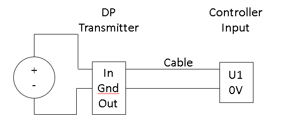
A differential pressure transmitter is powered by 24Vdc, providing an output of 0-10Vdc for a range of 0-4Bar. The sensor is connected through a run of cable 400 meters long, with a resistance of 30.5 Ω/km, to an input on a controller with an input impedance of 5kΩ. To start let me draw out the circuit:
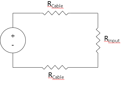
This circuit can be updated to a traditional electronic circuit as follows:
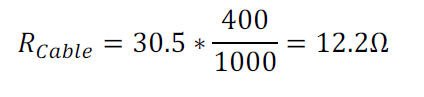
For a single core of the cable, the resistance is calculated as:
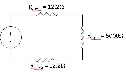
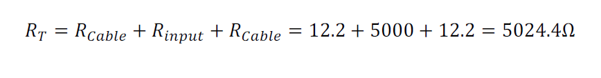
Now, we know the cable resistance and the resistance of the input, the circuit resistance can now be added:
The worst-case scenario for voltage drop will exist at the high end of the sensor range of 10Vdc. Our example will be based on this but you could equally base it on the maximum voltage you expect the transmitter to output. Using Ohms Law we can equate voltage, resistance and current.
We know the voltage of the circuit shall be 10Vdc and the circuit resistance is:
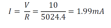
Current through the circuit, from Ohms Law, shall be:
Now that we have the current and we know the cable resistance we can calculate the voltage drop on the cable:
Therefore, using a cable with a resistance of 30.5 Ω/km to connect a water differential pressure transmitter providing 0-10Vdc output for a range of 0-4Bar connected to an input, 400 meters away, gives a voltage drop of 0.048Vdc at full range.
Following on from Part 2 of the series of converging BACnet networks, Part 3 will look at Virtual Extensible Local Area Network, which allow the BACnet network to be converged at the network switch level.
Virtual Extensible Local Area Network or VxLAN is an encapsulation protocol used to allow layer 2 packets to traverse the layer 3 boundary. VxLAN is most commonly found on network switches deployed in data centres where there are an extreme number of networked devices (servers) that may all have to site on a single converged network. In this way, VxLAN satisfies the needs of the data centre operator while also keeping all of the tenant servers on their networks. In larger commercial buildings you may find that the network switches located at the core support VxLAN, not by choice, but by function, while the switches out at the edge tend to be less expensive.
Without the use of VxLANs on a network with an extensive amount of BACnet devices, the design would have to be such that there is one large Layer 2 domain. All controllers would site on the one network under a single Layer 3 router. This may require the use of a Class A IP address which may not meet the network administrators requirements. Deploying a VxLAN allows layer 2 frames to be encapsulated into layer 3 packets and then routed as an IP packet across the network. Once the IP packet is received at the destination network, the network switch, removes the frame from the IP packet (de-encapsulation) and transmits it back out onto the network.
The VxLAN is a configuration carried out on the network switch and not all network switches, as noted previously, supports this functionality. The use of a VxLAN mitigates against the use of a BBMD on a BACnet network.
Following on from Part 1 of the series of converging BACnet networks, Part 2 will look at BACnet Broadcast Management Devices, which allow the BACnet network to be converged. In Part 1 there were four different broadcasts mentioned. Of these four only two would need to traverse the layer 3 boundary.
For the broadcast to traverse the layer 3 boundary a BACnet Broadcast Management Device or BBMD can be used. A BBMD can be a hardware device or a piece of software running a machine on each network. Where these are hardware devices that can standalone or the BBMD may be a function of your controller. As you will see there could be a lot of network traffic that could burden your controller so I would always recommend larger networks having dedicated BBMD devices.
The BBMD operates by taking the layer 2 broadcast frame and encapsulation it into a layer 3 IP packet. This IP packet is then routed across the network where the BBMD on the receiving network reverses this process and the broadcast frame is sent out to all devices.
Every subnet that requires the ability to broadcast messages from another subnet will require a BBMD. Therefore, there must be a BBMD on the subnet where the broadcast originates and a BBMD on the subnet where the message is to be directed.
Within the BBMD there exists a Broadcast Distribution Table or BDT. The BDT lists the IP address of all of the BBMD devices, including themselves, required to build the virtual converged network. There is a limit on the number of entries into a BDT therefore this must be considered while designing out your network.
Where a device, such as an operators workstation, sits on part of the network without a BBMD, these devices can still receive the broadcast through a mechanism called Foreign Device Registration or FDR.
Using the FDR mechanism the BBMD can forward a broadcast message as a unicast message. This mechanism operates as follows. The devices, which would require BACnet broadcasts, sends a request to a BBMD device that supports FDR. The BBMD device will record the details of the controller requesting BACnet broadcasts, into the Foreign Device Table or FDT. The entry into the FDT is stored for a finite amount of time and therefore the device requesting the forwarded broadcast must re-register at regular intervals.
In the final part of this topic, VxLan’s shall be discussed as a way to overcome the limitation of network broadcasts.
On larger networks where BACnet has been deployed, the routers can block some of the BACnet services. In this three-part post, I start by looking at where the problem lies with converging a large BACnet network and propose two solutions which will be discussed in the proceeding two blog posts.
How does layer 2 versus layer 3 on network switches and relate to the operation of BACnet? The BACnet specification defines several methods for the transmission of messages. These methods are:
Directed message sent from one device to another.
Local broadcast from one device to all other devices on the same network.
Remote broadcast from one device on a network to all devices on another network.
Global broadcast from one device on a network to all device on the internetwork.
Where a broadcast message moves from MS/TP to a BACnet/IP network, for example, this is not a problem, so long as the BACnet network is on a single subnet. If the BACnet/IP network is spread over multiple subnets there can be issues if the routers do not support bridging. A broadcast is a one to all device communication method. Several BACnet service such as ‘Who-Is’ and ‘I-Am’ rely on broadcast frames to communicate and build the network.
A broadcast frame will have the destination address as all binary ones or FF:FF:FF:FF:FF:FF. If a device receives this frame it will treat it as unicast and start to decode the frame. Where a device can receive a broadcast frame from another device it is said to be in the same broadcast domain. A broadcast frame is sent to every port except the originating port. The switch knows it is a broadcast package as every bit in the destination address is a one. BACnet broadcast uses frames operating at Layer 2 on the OSI reference model. Layer 2 frames are not routable on the network, only Layer 3 packets. Therefore BACnet broadcasts are contained in the same Layer 2 segment, as they cannot traverse the Layer 3 boundary.
Care should be taken with large BACnet networks, as these large networks are susceptible to Broadcast storms which can bring the network down and cause communications to fail. It may make sense to have different devices in different broadcast domains, for example, the primary plant may be on one network while all of your meters may sit on a separate network. A Layer 2 network switch can assign a Virtual LAN or VLAN to specific network ports, which are then in different Layer 3 subnets. The net result is that a switch can have multiple broadcast domains.
The issue may have become apparent at this stage. If multiple BACnet devices installed in a large building were there are multiple network switches in several different locations, these network switches will all be assigned different network addresses and all have separate broadcast domains. Given that the services that build a BACnet network operate on broadcasts if devices are all now on different broadcast domains, how can we bring the complete network online and allow for proper functionality? The answer to that question lies in different technologies. These are:
BACnet Broadcast Management Device or BBMD
Virtual Extensible LAN or VxLAN
Both of these technologies will be discussed in future blog posts and will be linked here
Following on from the last post discussing the use of mathematics within Building Management Systems Explained, the question of mathematics of control loop response analysis has been asked. This mathematics centres around the following techniques to help you understand how well a loop is tuned:
Integral of Absolute Error
Integral of Square Error
Integral of Time-Weighted Absolute Value of Error
Integral of Time-Weighted Error Squared
The best approach to discuss these techniques is to provide a pseudo code example of how these calculations can be carried out. Before I create this code I need to speak to absolute values.
The absolute value is the non-negative value without regard for the sign. |Value| is defined as the absolute value. Therefore, if Value is a negative number, |Value| is always a positive number.
I will show an example of how to calculate the Integral of Absolute Error and pseudo code for the other three integral methods. From the initial example and pseudo code of other methods, you should be able to calculate these values for your own data sets.
Integral of Absolute Error
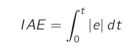
Integral of Absolute Error, or IAE, is calculated as follows:
The pseudo code to calculate the Integral of Absolute Error is as follows:
Set a Counter to iterate from the second position to the last position.
   |Previous Error| = Previous Process Variable – Previous Setpoint
   |Current Error| = Current Process variable – Current Setpoint
   Time Difference = Time of Current Error – Time of Previous Error
   IAE = IAE + (Time Difference/2)•(|Previous Error| +|Current Error|)
Iterate Counter
In reality how does this pseudo code operate? Let us look at an example:
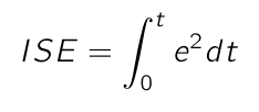
Integral of Square Error, or ISE, is calculated as follows:
The pseudo code to calculate the Integral of Square Error is as follows:
Set a Counter to iterate from the second position to the last position.
   |Previous Error| = Previous Process Variable – Previous Setpoint
   |Current Error| = Current Process variable – Current Setpoint
   Time Difference = Time of Current Error – Time of Previous Error
   ISE = ISE + (Time Difference/2)•(square(|Previous Error|) +
                                               square(|Current Error|))
Iterate Counter
Integral of Time-Weighted Absolute Value of Error
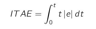
Integral of Time-Weighted Absolute Value of Error, or ITAE, is calculated as follows:
The pseudo code to calculate the Integral of Time-Weighted Absolute Value of Error is as follows:
Set a Counter to iterate from the second position to the last position.
   |Previous Error| = Previous Process Variable – Previous Setpoint
   |Current Error| = Current Process variable – Current Setpoint
   Time Difference = Time of Current Error – Time of Previous Error
   Time Since Start = Time of Current Error – Time of Since Start
   ITAE = ITAE + (Time Difference/2)•(Time Since Start•|Previous Error|
                                      + Time Since Start•|Current Error|)
Iterate Counter
Integral of Time-Weighted Error Squared
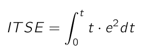
Integral of Time-Weighted Error Squared, or ITSE, is calculated as follows:
The pseudo code to calculate the Integral of Time-Weighted Error Squared is as follows:
Set a Counter to iterate from the second position to the last position.
	|Previous Error| = Previous Process Variable – Previous Setpoint
	|Current Error| = Current Process variable – Current Setpoint
	Time Difference = Time of Current Error – Time of Previous Error
        Time Since Start = Time of Current Error – Time of Since Start
	ITSE = ISTE +
           (Time Difference/2)•(Time Since Start•square(|Previous Error|)
                              + Time Since Start•square(|Current Error|))
Iterate Counter
I have been asked over the last week about the mathematical symbols used within the book. I had toyed with the idea of having an additional Appendix within the book to discuss the mathematics spread throughout the chapters. In retrospect, looking at the number of questions I have had about mathematics, an Appendix would have been prudent.
One of the first points of confusion may be the use of a dot for multiplication. The dot operator is used within mathematics to avoid confusion. For example, c • 3 is used to avoid confusion with c3. Similarly, with algebraic equations, the x symbol for multiplication could be confused with a variable. For example:
y = m • + c
is much less confusing than:
y = m x x + c
The question has been asked as to why the asterisk (*) symbol was not used to denote multiplication. While this is typical for use in programming languages, this symbol does not form part of normal mathematics. After some investigation, historically, the * symbol was used to denote factorial. Factorial, written as n! or historically n, where n equals 5 yields the following results:
5! = 5 • 4 • 3 • 2 • 1 = 120
The next two symbols I have been asked are the sum (Σ) and the product (Π) symbols. Let me start with the sum or Σ symbol. The symbol Σ is the Greek letter sigma and is used to denote a sum of multiple terms. Sigma is usually accompanied by an index which spans the range of values that should be considered in the summation.
Where n is the index of summation, a is the index of the first value of n, b is the index of the last value of n and f(n) is the function carried out on n as part of the summation.
I know this may seem confusing but let me work through a few examples for you. First I must define a data set. Let us use the numbers one to five as our dataset:
1, 2, 3, 4 ,5
To start let us look a simple example:
The mathematical equation here is the sum the values from the first number to the fifth number. Therefore,
1 + 2 + 3 + 4 + 5 = 15
So imagine now the following equation:
The mathematical equation here is sum the values from the second number to the fourth number. Therefore,
2 + 3 + 4 = 9
Pretty straight forward so far. Now imagine n as a formula. A simple example would be:
The mathematical equation here is sum of double the values from the first number to the fifth number. Therefore,
2 • 1 + 2 • 2 + 2 • 3 + 2 • 4 + 2 • 5 = 30
Hopefully, now you have an understanding of the summation notation. Next, let us look at the product notation. We will not look at as many examples. The symbol Π is the Greek letter Pi and is used to denote a product of multiple terms. Pi is usually accompanied by an index which spans the range of values that should be considered in the product.
Where n is the index of product, a is the index of the first value of n, b is the index of the last value of n and f(n) is the function carried out on n as part of the product.
Thinking back to our data set of 1, 2, 3, 4, 5 consider the following example:
The mathematical equation here is the product of the values from the first number to the fifth number. Therefore,
1 • 2 • 3 • 4 • 5 = 120
The product operates the same as the summation, but instead of adding the values you are multiplying the values. The rules are the same.
I hope this post has helped with some of the questions around the mathematical notation used in the book. The next post will focus in on the intagration techniques that are spoken to in Chapter 4 on control theory.
I am delighted to announce, I got my first book finished and published and available on Amazon. Building Management Systems Explained: Understanding Controllers and Field Devices explains the controller hardware and commonly used field devices. Building upon first principles of electrical, electronic, controls theory, psychrometrics, networks plus protocols and field devices. The reader will gain the knowledge required to specify, design, install, commission or troubleshoot a BMS. This book is aimed at Engineers of all levels and provides worked examples in many areas.
Due to the current pandemic, Amazon is only shipping in-region in Europe, so if you are looking for a hard copy, head over to Amazon.com. For Kindle readers, as this is a technical book with a lot of schematics, tables and equations, this book is only readable on the Kindle app on smartphone or tablet and not on a Kindle device.